15418_mesh_project
The Application of CUDA and openMPI in Mesh Simplification
Alejandro Gonzalez Lazaro (alejand2) and Majd Almudhry (malmudhr)
SUMMARY:
We will implement the mesh simplification algorithm by Michael Garland and Paul Heckbert on the GHC machines’ multicore processors and GPUs. The two implementations require different strategies that we will compare in this paper.
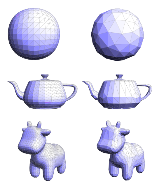
Credit: https://github.com/CMU-Graphics/Scotty3D/blob/main/assignments/A2/simplify.md
BACKGROUND:
The project is about using a mesh simplification algorithm developed at CMU by Michael Garland and Paul Heckbert. From the 15462 assignment, the pseudo code for the algorithm looks like the following:
- Compute quadrics (a matrix whose details are in the webpage listed in the resources) for each face.
- Compute an initial quadric for each vertex by adding up the quadrics at all the faces touching that vertex.
- For each edge, create an Edge_Record (a data structure) and add it to one global queue.
- Until a target number of triangles is reached, collapse the best/cheapest edge (as determined by the queue) and set the quadric at the new vertex to the sum of the quadrics at the endpoints of the original edge.
Here we will go over some of the key parts of this algorithm.
Key data structures: The Halfedge Mesh data structure is made up of lists of the following 4 different Elements.
-
Edge: contains pointers to a halfedge
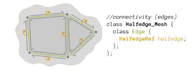 Fig 2: Credit: https://github.com/CMU-Graphics/Scotty3D/blob/main/assignments/A2/halfedge.md
 -
Face: contains a pointer to a halfedge
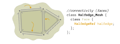 Fig 3: Credit: https://github.com/CMU-Graphics/Scotty3D/blob/main/assignments/A2/halfedge.md
 -
Vertex: contains the position of the vertex and a pointer to a halfedge
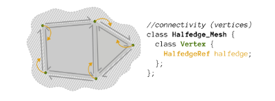 Fig 4: Credit: https://github.com/CMU-Graphics/Scotty3D/blob/main/assignments/A2/halfedge.md
 - Halfedge: contains corner uv and normal data and pointers to most of its connectivity in the mesh:
- A twin halfedge, a next halfedge, a vertex, an edge and a face
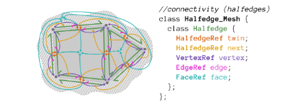 Fig 5: Credit: https://github.com/CMU-Graphics/Scotty3D/blob/main/assignments/A2/halfedge.md
- A twin halfedge, a next halfedge, a vertex, an edge and a face
- 2 unordered maps
- A vertex reference to quadric matrix map
- A face reference to quadric matrix map
- A priority queue of edge records where each record stores:
- A reference to an edge, its cost, and the optimal position of the new vertex that will replace it after collapse
Key Operations on Data Structures:
-
The Collapse Diamond structure: When we collapse an edge, the mesh area around the edge (Bolded Blue) needs to be modified. Components of the halfedge data structure marked with a red cross need to be deleted and magenta arrows represent references that need to be switched to other components.
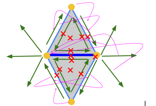 Fig 6: Collapse Diamond
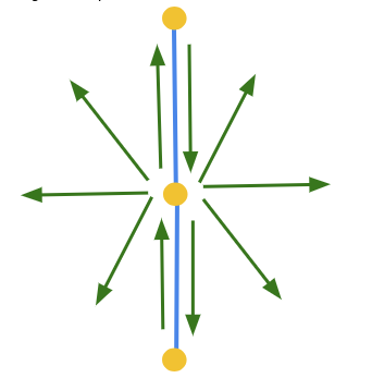 Fig 7: Collapse Diamond after Edge Collapse
 -
Unordered Maps: For each face in the mesh, a quadric matrix needs to be computed and stored once, then for each vertex a quadric matrix is computed by summing up all the quadric matrices of the faces surrounding it. These matrices are used to compute the cost of collapsing each edge and the new optimal position for the replacing vertex. Thus, whenever a new vertex is created a new quadric matrix should also be added to this dictionary. Edge Record Priority Queue: Every time we want to collapse an edge we need to pop off one edge from the top of this queue which stores edges by cost. Then, before we collapse an edge we take out every surrounding edge’s record and place it back in the edges surrounding the new vertex that has replaced the previous edge.
Algorithm’s Inputs and Outputs: The algorithm takes in a halfedge mesh data structure and outputs another halfedge mesh data structure (these are generally stored in js3d files, but file loading/saving these files is outside the scope of our algorithm). What is the part that is computationally expensive and could benefit from parallelization? The computation of quadrics per face, vertex and edge can be parallelized The collapse of edges can be parallelized when there are no conflicts with other parts of the mesh that are being collapsed simultaneously.
Workload Breakdown.
Intrinsically, the halfedge mesh has a large amount of parallelism that can be accomplished; different parallel elements do not modify elements that other elements need to access/modify. For instance, outside of the Collapse Diamond area that we described above, another parallel unit can collapse any edge that does not touch any of the elements in another’s Collapse Diamond area. This can amount to good data parallelism if conflicts are detected and handled appropriately. Moreover, there is potential for temporal locality while computing an edge collapse, but not as much space locality as the halfedge mesh structure is stored as a set of references between items.
APPROACH
- Technologies Used: This project runs on top of Scotty3D (https://github.com/CMU-Graphics/Scotty3D) a 3D modeling, rendering and animation program for 15462 assignments. This program is written in C++ and we introduced MPI and cuda components for our parallelization. Our main target was the 8-core multiprocessor and NVIDIA 2080 graphics cards found on the GHC clusters. Mapping the Problem in Parallel
- MPI: To simplify our mesh in parallel, our aim was to assign a section of the mesh to each of the MPI processes. Each section or sub-mesh should minimize the amount of overlap with other sub-meshes owned by other processes. This way, we can avoid conflicts with other collapses done by other processing elements as much as possible.
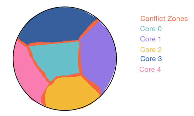 Fig 8: Mesh Partitioning for MPI
When we partition our mesh, we traverse over every edge and attempt to save all the data in the Collapse Diamond that we need for collapsing that edge to that partition and set the owner of that element to it. If some of that data is already owned by another partition, we will still add the element to the partition but we will not update the owner. This will function as a “ghost cell”. Any edge that is linked to ghost cells will now become part of the “conflict zone” where collapsing cannot be done without communication as there exists data owned by someone else there. The data in each partition is determined by iterating over every edge and carrying out a breadth-first search of other edges, to maximize the area to the conflict zone perimeter. In our current implementation, we first compute the partitions from a master process and asynchronously send each of the halfedge, edge, vertex, and face arrays to each process. From here, each process (including the master process) takes its respective partition data and begins simplification. From here, we handle edges in the conflict free zone by first checking the Collapse Diamond data structure and if no conflicts are found with data owned by other partitions we commit to collapsing the edge. After each of the processes collapse their respective number of target edges, these partitions are communicated back to the master process asynchronously. This main process is assigned edges last so it has less work to do than the other processes so it is ready to receive each piece of data from the other processes. We send each array from each process individually and asynchronously so that the main process can update the main mesh as data is coming in and not at the end while waiting for everyone to send their data.
- CUDA:
Adapting original data structures for parallelization:
As we have already mentioned, the halfedge data structure is built up of a series of references to the different elements around the mesh. The problem with this design is that the two parallelization models that we chose require memory transfers between devices that are not in the same shared memory system. Thus simply transferring the original data structures across devices would render all those pointers useless. As such, we changed all of the base data structures such that instead of using element pointers (ElementRef) they would store uint32_t indexes into each array of halfedges, faces, vertices and edges, so that any previous element dereference would be converted into an array access. With this, transferring each of the arrays over with MPI and between CPU and GPU became possible. For both CUDA and MPI implementations, we begin by translating the loaded halfedge mesh into our array version. This conversion is not included in our initialization time as the mesh is loaded into the original reference based halfedge data structure but in our encapsulation of our testing we assume that it’s already in the right format. The following are some of the additional modifications we made per implementation:
- MPI: To keep track of elements across partitions, we have to expand each of the element data structures. Each reference to another connected element now includes two separate uint32_t indexes, one global index (which represents the index in the final global mesh array) and one local index (which represents the index in the current partition’s array). We also keep track of the owner of the referenced elements and also the current owner of this element to check for conflicts and for potential communication of collapses that concern ghost cells so that all the different owners can get involved.
- CUDA: The main changes made to the data structures with CUDA besides the translation to arrays has to do with C++ STL since they cannot be used inside a CUDA kernel. This meant that we had to find a replacement for every standard library function that we used such as rand(). We also added markers on each element to indicate who the thread owner of that element is. Iteration Process: In this section we will first talk about the improvement process to our current algorithms and then about some ideas we attempted to implement but had to leave behind.
-
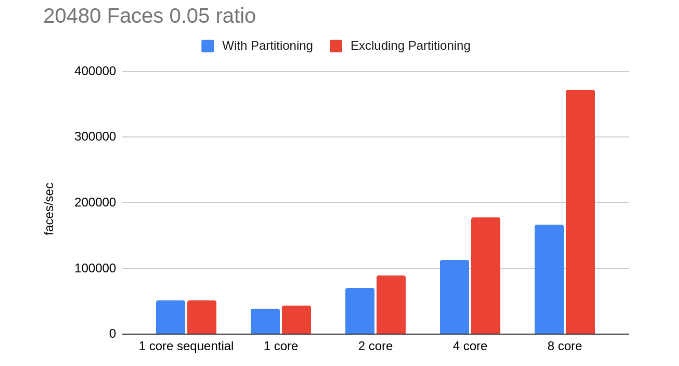
MPI: In our initial MPI implementation we had a simple broadcast of the partition arrays and then a synchronous receive of all the finished partition data. To improve this, we changed the broadcast and gather stages to use asynchronous sends and receives. This way, the master process does not need to wait for other processes to receive their partitions before it starts to work, and then it can do work (rebuilding the final mesh), as it receives data asynchronously from the other processes. These changes helped bring down the communication time somewhat but the biggest bottleneck in our design was the initial partitioning stage. For instance here is our data before some optimization of the partitioning stage with a sphere consisting of 20480 faces:

This speedup happened after we did some restructuring and removing inefficiencies in the code. This partitioning step is inherently serial but some of the later steps after the breadth first search assignment could be parallelized thus we attempted to parallelize that later step but between the extra communication and necessary steps to adapt to these last steps the time delta was not consistently better thus we kept the whole partitioning serially.
- CUDA The main challenge with the CUDA algorithm is the synchronization that is required across all threads in a grid. If the algorithm was to be implemented on a CPU, then using locks would have been a possible solution to prevent conflicts. However, CUDA does not provide a simple mechanism for a general mutex lock. Also because of warp execution, deadlocking is hard to avoid and is what we struggled with in our initial approach. That’s why we decided to use an approach that is similar to a lock-free implementation that marks an element, synchronizes with all running threads, and then checks the mark again. Another challenge with working with GPUs in general is the high cost of accessing global memory. However, given the nature of the huge data structures we’re using, copying everything to shared memory is not possible. One thing that helped with that is removing the vertex quadrics which is an array of 4x4 matrices of flouts the size of the vertices. This is a performance-space tradeoff as having that array around saves us from having to compute the quadric cost every time we collapse an edge, but given how huge of a space that array takes, it was the better decision to get rid of it. We have tried doing that with a smaller mesh, and it produced the following results. We can clearly see how shared memory is much faster than global memory as it takes an order of magnitude less even for a small mesh.

However, we again ran out of shared memory as we used bigger meshes. So, a better approach would be to partition the mesh, similar to how it’s done with MPI, and make every block handle a different partition. However, we were not able to fully test this approach yet.
One issue we faced throughout our time with this project was that there seems to be a bug in our sequential version of the algorithm that we could not find. Our theory is that when we handle an edge collapse once, this produces a valid mesh but some reference change is not quite right. Thus if we collapse edges around an area we had collapsed before, this error can compound and eventually produce an invalid mesh. As a result in some cases we were not able to generate valid meshes, and often found our code running into infinite loops when traversing the mesh due to mesh inconsistencies. Hence here we will talk about some of the improvements we began to implement/planned for our parallelization but were hindered by this bug.
- MPI:
- Handling Conflict Zones:
In the current implementation, we just handle edges outside of the conflict zone. However we had some ideas to be able to handle collapsing edges with items in the Collapse Diamond found in ghost cells.
To be able to handle conflicts, we decided to implement a transaction-based system where changes to the Collapse Diamond are stored first, marked for conflicts with other partitions and committed/aborted depending on certain conditions which we will detail here:
- No other dependant partitions are found: In this case the transaction can be committed without communicating with any other process.
- Dependants are found but this partition owns everything in the Collapse Diamond (Full Owner Case): The transaction is committed, but we send the data for the transaction to every dependent thread so that they can update their own data structures.
- The Collapse Diamond contains elements owned by other processes: In this case, we check if previously committed Full Owner transactions conflict with the current transaction and abort it if it does, otherwise, we send a message to all the other processes (and check for messages from others), so that a synchronization event can happen. When all threads come together, they will all check all pending transactions in some arbitration order and the owners of each piece of data will approve or deny the transaction if no conflicts are found, then each of the processes will bring in the transaction data into their own data structures. In our implementation we began with creating the transaction mechanism to handle the first two cases. However, it seems that with this strategy the bug we have discussed before showed its head again and generated invalid meshes, thus we spent many days attempting to find the bug and implementing the transaction mechanism in different ways but were not able to get it to work. There is also another potential issue with this strategy for the conflict case. Currently, as we are only deleting elements in our local element arrays, we can keep our array sizes constant. Nevertheless, If we delete edges in the conflict zone, we need to bring in the surrounding area to the removed edge and generate new ghost cells for each process. This raises a new problem. This would require us to communicate neighboring data, apart from the data found in the transaction diamond, from each of the owners of elements in the transaction to each of the dependents of the transaction. This is also the uncertainty as to how much neighboring data needs to be communicated to each different dependent so that they have complete ghost cells, and this can easily spiral out of control if we pick edges from the conflict zone too frequently.
- Handling Conflict Zones:
In the current implementation, we just handle edges outside of the conflict zone. However we had some ideas to be able to handle collapsing edges with items in the Collapse Diamond found in ghost cells.
To be able to handle conflicts, we decided to implement a transaction-based system where changes to the Collapse Diamond are stored first, marked for conflicts with other partitions and committed/aborted depending on certain conditions which we will detail here:
- CUDA CUDA: To run the same algorithm using GPUs, we used a different implementation that is more suited to the architecture of a GPU. We referenced this paper in our approach with CUDA to simplify the process. So after we copy all the data structures over to the global memory of the GPU, we run one kernel to compute the vertex quadrics, and then run another kernel that does all the simplification. There are two phases in that second kernel. During the first phase, all threads in a block randomly choose a potential edge to collapse, and then after all threads are done, the edge with the minimum cost is selected. In the second phase, if the selected edge in the first phase is not dead (already collapsed), then all elements (vertices, halfedges, etc. ) in its critical area are marked with the ID of the thread that’s trying to collapse it. All threads across all blocks are then synchronized. Across block synchronization is not trivial in CUDA, but can be achieved with a feature called cooperative groups that was released as part of CUDA 9.0. After every thread in a block marked its elements, they’re checked again for no corruption to ensure no other thread picked a conflicting edge. If the marks were not corrupted, and thus all threads picked independent edges, then the thread proceeds to collapse that edge. The process is repeated until a specific ratio is achieved after which everything is copied back to CPU and the mesh is validated.
RESULTS
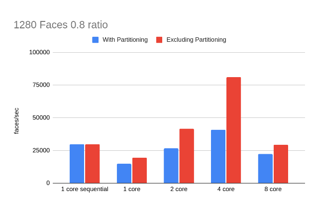
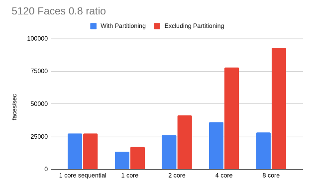
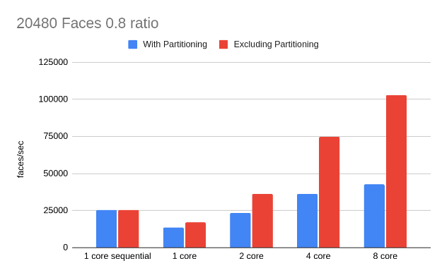
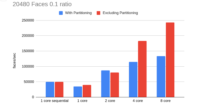
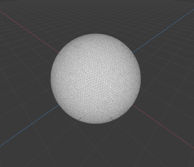
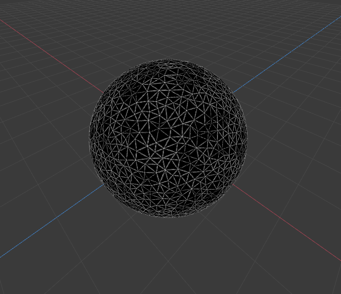
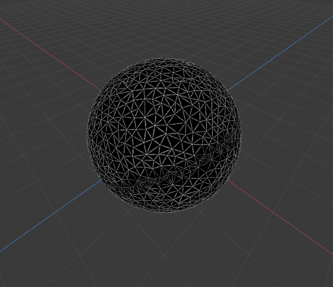
To test our implementation we have generated some sphere meshes of different face counts and simplified them with different ratios. We will compare our results both with our original sequential code and the single core performance of our parallel code. We will measure our performance in triangles collapsed per second. As we will see in all the following results, partitioning can be a bottleneck. However, the partitioning has to be done once and its cost could be amortized if we reuse it if we need to simplify a mesh multiple times at multiple resolutions (For example when the mesh is seen on the screen from multiple different distances), hence we will also show the speedup without the partitioning cost.
-
MPI

Sample renders from 20480 Faces Sphere with 0.2 ratio
- Original mesh
- 1 proc
- 2 procs
- 4 procs
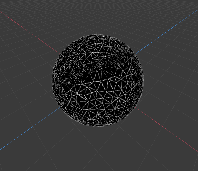
- 8 procs
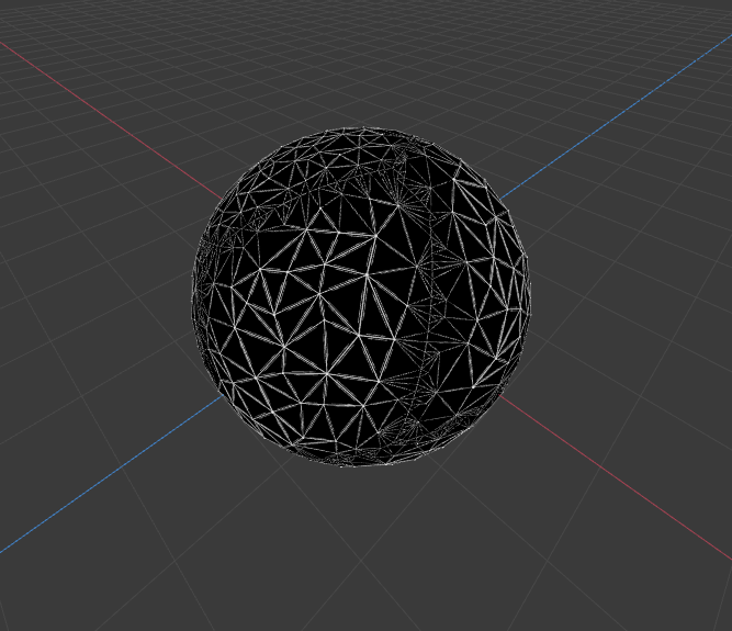
- Original mesh
-
CUDA
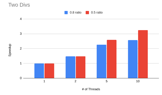
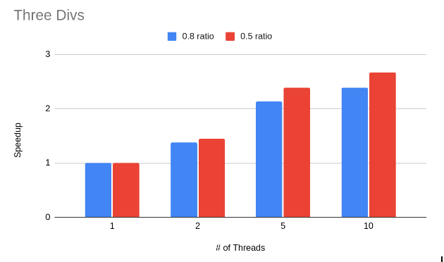
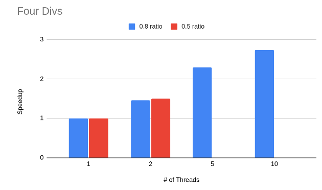
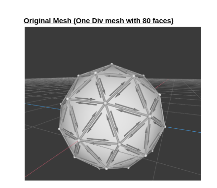
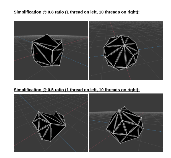
DISCUSSION
-
MPI We can see throughout our results that our main limitation for speedup was the partitioning step since this is inherently sequential. However, this step is very useful when it comes to avoiding conflicts in our edge collapse (our code currently searches for edges outside of the conflict zone thus seeing near linear speedup shows us that we are able to find non-conflict edges more often than not). Thus, next optimization efforts should focus on other partitioning methods as the kd-tree method that we had planned to reduce that overhead. Still, we can see that higher mesh sizes and lower ratios of simplification (smaller mesh at the end) are able to amortize the extra partitioning cost and achieve better speedup. The following is an example analysis of execution time for the 20480 0.05 8 core simplification case, as we can see partitioning takes more than half the execution time:

We can see that choosing a multicore processor was a good idea to speed up mesh simplification, however, using MPI instead of Shared Memory may not be the best for consumer targeted multiprocessors (which is our intended use case) as this required a large amount of reworking of structures to be transferable through memory and made conflict zone collapse more complicated to implement than potentially making use of locks only at conflict zones. Would be interesting to try this algorithm with OpenMP instead of OpenMPI.
-
CUDA There are two main problems with the CUDA implementation which might explain why the speedup is far from ideal. The first problem is the small problem size. Only smaller meshes with high ratios worked with CUDA because of the cost computation bug that we have. This makes it harder to draw a conclusion on how effective this approach is. The second problem is inherent to the algorithm chosen here. After the kernel is done from its first phase, where it chooses a single edge to collapse, every other thread in the block remains idle as it waits for that thread to finish collapsing the edge. Clearly there’s a better way to better utilize all the GPU resources. We think looking at algorithms such as the one with the priority queue that we talked about in our milestone report would be interesting. The reason we didn’t use that approach is because of our problems with the sequential implementation that we thought a simpler approach would be easier to debug and analyze. The following tables show some analysis of execution time for the two main phases in the CUDA kernel in units of clock cycles.

We can see from these results that we need to find a way to parallelize the second phase more or find things to overlap with during that time.
RESOURCES
- https://github.com/CMU-Graphics/Scotty3D
- https://github.com/CMU-Graphics/Scotty3D/blob/main/assignments/A2/simplify.md
- https://www.cs.cmu.edu/~./garland/quadrics/quadrics.html
- https://www.ncbi.nlm.nih.gov/pmc/articles/PMC8341488/
- https://en.wikipedia.org/wiki/Breadth-first_search
- https://journals.plos.org/plosone/article?id=10.1371/journal.pone.0255832
SCHEDULE:
Week 0 (March 24-31): (DONE)
Get the Scotty 3D build system compiling CUDA and MPI and start sequential implementation.
Week 1 (April 1-7): (DONE)
Finish sequential implementation
Week 2 (April 8-14): (DONE)
Sketch out the algorithms for both CUDA and MPI and start implementing them.
Data structure reworking
MPI Partitioning
Week 3.1 (April 15-17):
Implement edge record pass for MPI (Alejandro) (DONE)
Start implementing the “relaxed priority queues” for CUDA (Majd)
Week 3.2 (April 18-21):
Implement collapsing pass for MPI (Alejandro) (DONE only with non-conflicts)
Finish implementing the “relaxed priority queues” for CUDA (Majd)
Week 4.1 (April 22-24):
Implement gather and rebuild from partitions for MPI (Alejandro) (MOVED)
Implement the locking part for CUDA (Majd)
Week 4.2 (April 25-28):
Implement gather and rebuild from partitions for MPI (Alejandro) (DONE) Add collapsing for MPI with conflicts (Alejandro) (DONE)
Partitioning algorithm with CUDA (Majd)
Week 5.1 (April 28-May 1):
MPI alternate mesh partitioning with KD-trees (Alejandro)
Optimization/Data collection CUDA (Majd)
Optimization/Data collection MPI (Alejandro) (DONE)
Edge collapsing for partitioning algorithm (Majd & Alejandro)
Week 5.2 (May 2-May 5):
Poster and report (Alejandro & Majd)
PROPOSAL URL:
https://docs.google.com/document/d/13vQRTEH8dcyKOkdxwu2RBkG24wPOiYFiHQDjRZhcpcI/edit?usp=sharing
PROJECT MILESTONE REPORT URL:
https://docs.google.com/document/d/1yHcyYbR6AOp56O6Ecy0u2nk4vsgWCoEUkRCMBGLWxfk/edit?usp=sharing
FINAL REPORT URL:
https://docs.google.com/document/d/17UkdbUonFj9XmygbsjkXXH3oLB5dvahuskbuaYc_oZU/edit?usp=sharing